Applied ML · Forecasting

GridCast AI

Forecasts Great Britain’s half-hourly electricity demand 48 hours ahead from NESO’s 2024 record, serves the model through a typed FastAPI service, and explains each prediction with SHAP.

Model: Linear Regressionscikit-learn, with SHAP explanations
API: FastAPI on RenderServes the saved 2024 record, not a live feed
Interface: Next.js on VercelDashboard validates every API response
Evaluation: 1.36% MAPE, one step aheadHeld-out data; no 48-hour backtest yet
Links: Live demo Source

The served model’s 48-hour forecast. The shaded band is approximated from validation RMSE; it is not a calibrated per-step interval.

The problem

Electricity cannot be stored at grid scale, so supply has to be scheduled against demand that has not happened yet. Across 2024, Great Britain’s national demand ran from about 15 GW to 45 GW, and it moves by several gigawatts within a single day. A short-horizon forecast is the input every scheduling decision depends on.

GridCast is a complete forecasting system built around that problem: ingestion and validation of the public NESO record, feature engineering, model comparison on a held-out period, a serving API, an analytics dashboard and per-prediction explanations. The aim was a system whose numbers can be traced and whose limits are stated, not a model in a notebook.

From raw record to features

The loader checks the expected columns, keeps settlement periods 1–48 (clock-change days have 46 or 50), builds timestamps and reindexes onto a continuous 30-minute grid.
Validation runs before and after feature building, checking gaps, duplicates, nulls, negative demand and ordering, and fails the pipeline if either report has issues.
Eleven features: calendar (hour, day, month, day of week, weekend), demand lags at 30 minutes, one day and one week, and rolling means over 3, 48 and 336 periods, shifted so a row only ever sees the past.
The first week is dropped where lags are undefined, leaving 17,232 modelling rows from 17,568 raw rows.

Leakage kept out by whitelist: Two columns in the NESO file, transmission system demand and England & Wales demand, describe almost the same quantity as the target. Training reads an explicit list of eleven features, so they can never reach the model.
A chronological split, no shuffling: The first 80% (13,785 rows, to 21 October 2024) trains the model; the last 3,447 rows, to 31 December, are held out. Random shuffling on a time series would leak the future into training.

Evaluation, measured honestly

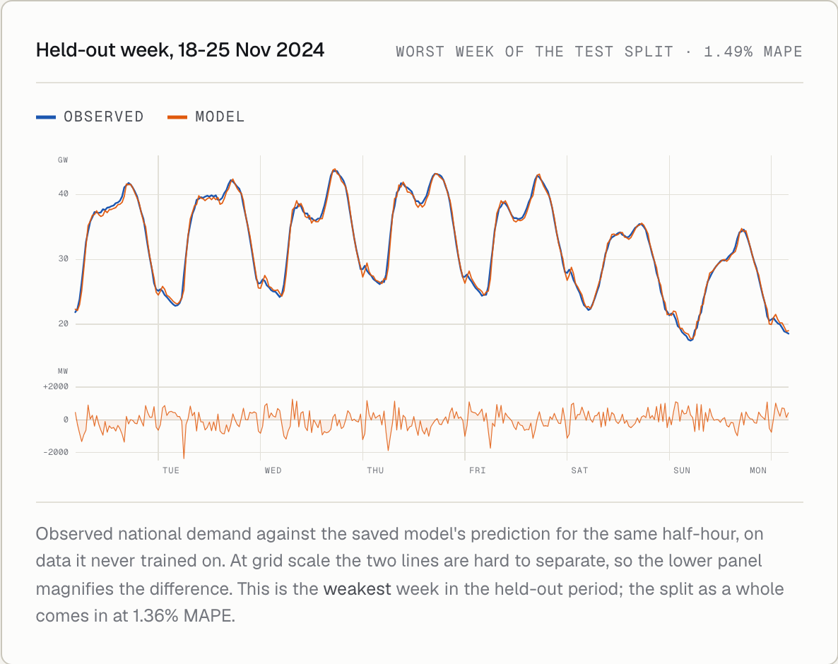
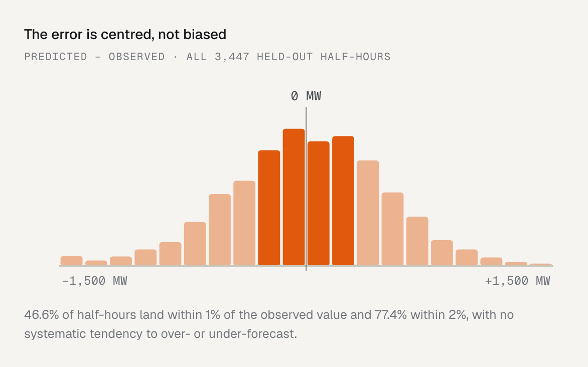
Two baselines were scored on the same held-out window and the lowest RMSE was served. Linear Regression won by 0.15 MW of RMSE (492.0 against 492.2), while Random Forest was slightly better on MAE and MAPE. The system serves the simpler model and says so, rather than presenting the choice as clear-cut.

held-out MAPE, one step ahead: 1.36%; held-out MAPE, one step ahead
held-out MAE, one step ahead: 386 MW; held-out MAE, one step ahead
held-out R²: 0.9936; held-out R²
MAPE in the worst held-out week: 1.49%; MAPE in the worst held-out week

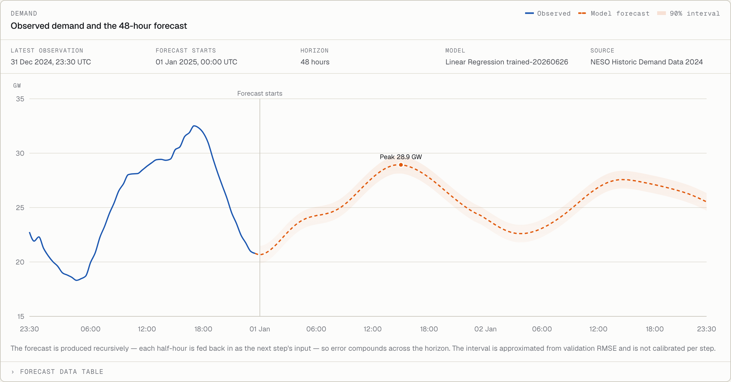
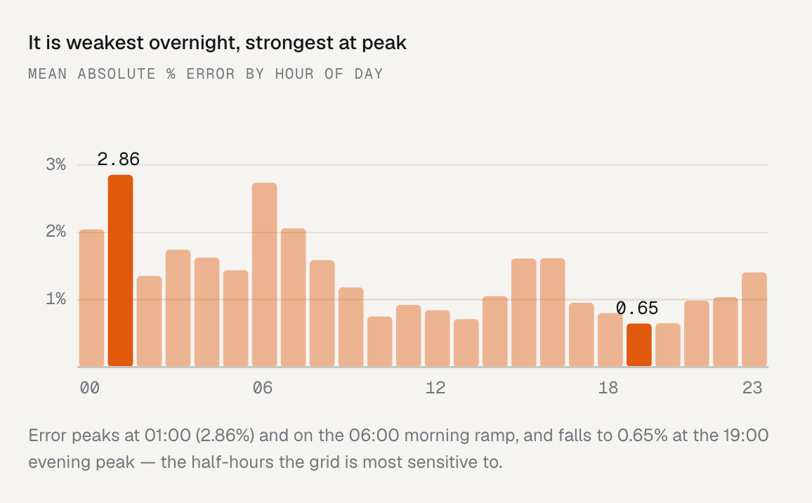
All of these are one-step-ahead measurements: each prediction sees the real previous half-hour. The 48-hour forecast feeds its own predictions back in for 96 steps, so error compounds across the horizon, and that horizon has not been backtested yet. The site never presents one-step accuracy as 48-hour accuracy.

Held-out week of 18 to 25 November 2024: observed and predicted demand overlap closely, with the residual magnified in a lower panel. Worst week of the test split at 1.49% MAPE. — The weakest week in the held-out period, observed against predicted for the same half-hour, with the error magnified underneath.

Histogram of held-out residuals centred on zero. — Held-out error is centred rather than biased, and is weakest overnight (2.86% at 01:00) and strongest at the evening peak (0.65% at 19:00).

Mean absolute percentage error by hour of day: highest overnight around 01:00, lowest at the evening peak around 19:00. — Held-out error is centred rather than biased, and is weakest overnight (2.86% at 01:00) and strongest at the evening peak (0.65% at 19:00).

Serving and explaining

Pipeline
Python · scikit-learn
Ingestion, validation, features, training and comparison, saved as one model artifact plus metadata.
API
FastAPI
Forecast, history, metrics, model, feature importance, per-prediction explanation and scenario endpoints.
Explainability
SHAP
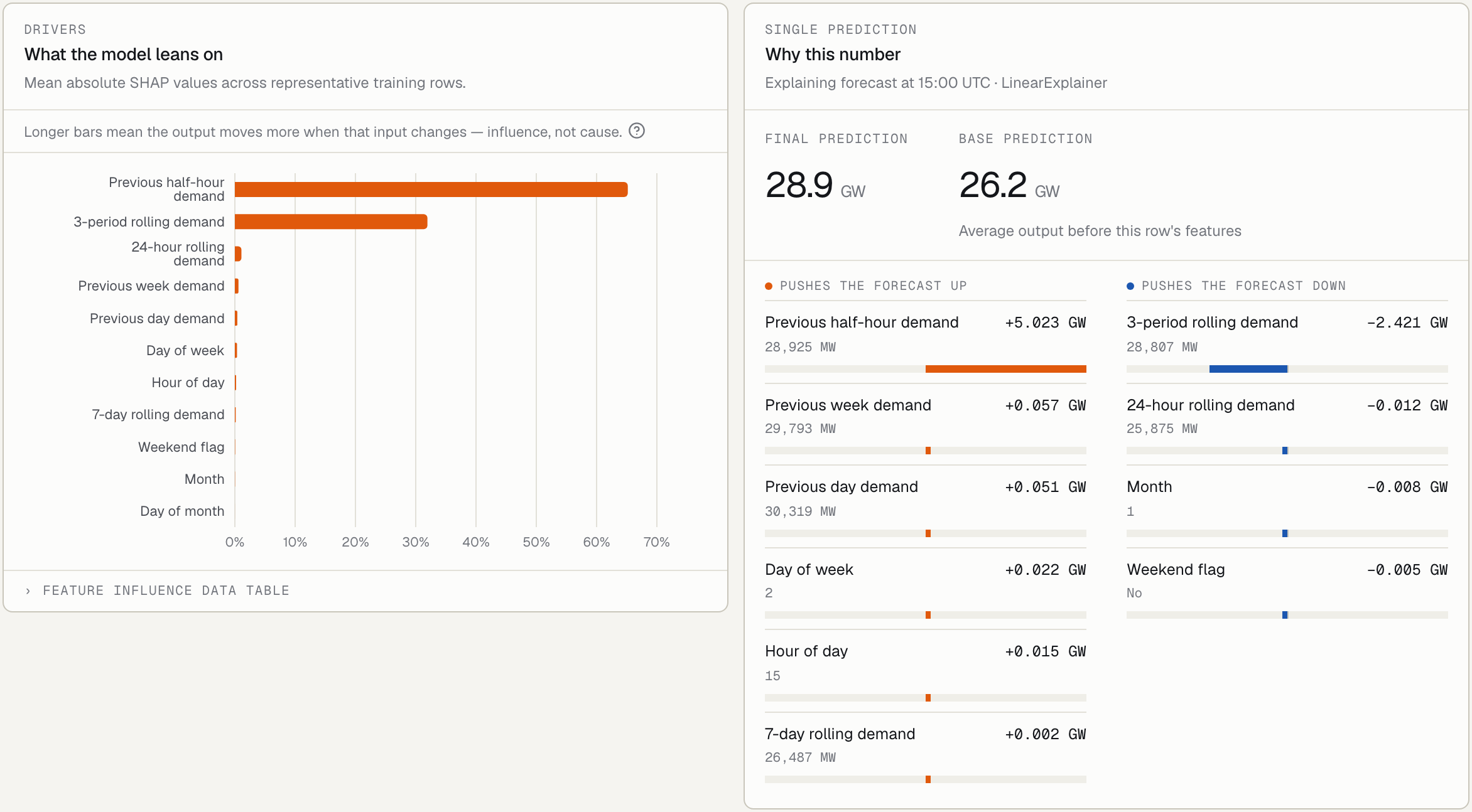
LinearExplainer over 256 background rows: global importance and a local breakdown for any forecast step.
Dashboard
Next.js · TypeScript
Server-side fetches with five-minute revalidation and runtime shape checks on every response.

Every response says where it came from: API responses carry a data source of artifact or fallback, and the dashboard refuses fallback data instead of showing placeholder numbers as real.
Precompute and cache against the artifact: The 96-step forecast is computed at startup, and caches are keyed on the artifact’s path, modification time and size, so a retrained model invalidates them automatically.
Pin the runtime to the model: scikit-learn is pinned to the version that pickled the model, after real dependency and Python-version conflicts during deployment.

GridCast model insights. Left: mean absolute SHAP values across representative training rows, dominated by previous half-hour demand and the 3-period rolling mean. Right: the 15:00 forecast explained, a final prediction of 28.9 GW from a 26.2 GW base, pushed up 5.0 GW by previous half-hour demand and down 2.4 GW by the 3-period rolling mean. — Global influence across training rows, and the breakdown of one forecast from the served model. Both show it leans almost entirely on the last few half-hours of demand.

38 backend tests (pytest) cover the data pipeline, training, the inference API and the runtime cache. The frontend relies on type-checking, linting and the production build.

Limits

Weather, holidays and generation mix are not model inputs.
It runs on a frozen 2024 record; it is not connected to a live NESO feed.
The 90% band is ±1.645 × validation RMSE at every step, so it is not calibrated per horizon.
The 48-hour horizon has no rolling-origin backtest; only one-step accuracy is measured.
The scenario simulator scales lag features with hand-set factors, and regional map layers are illustrative allocations of the national figure, labelled as such in the app.